Introduction

A discharge rating curve is a model that describes the relationship between water elevation and discharge in a river. The rating curve is estimated from paired observations of water elevation and discharge and it is used to predict discharge for a given water elevation. This is the main practical usage of rating curves, as water elevation is substantially easier to directly observe than discharge. This R package implements four different discharge rating curve models using a Bayesian hierarchical modeling framework:

plm0() - Power-law model with constant log-error variance.
plm() - Power-law model with stage-dependent log-error variance.
gplm0() - Generalized power-law model with constant log-error variance.
gplm() - Generalized power-law model with stage-dependent log-error variance.

For further details about the different models, see Hrafnkelsson et al. (2022). For an brief overview of the underlying theory, see our Background vignette.

The models differ in their complexity, gplm being the most flexible and complex model. We will focus on the use of gplm throughout this introduction vignette and explore the different ways to fit the gplm and visualize its output. However, the API of the functions for the other three models are almost identical so this vignette also helps users to run those models.

> library(bdrc)
> set.seed(1) #set seed for reproducibility

We will use a dataset from a stream gauging station in Sweden, called Krokfors, that comes with the package:

> data(krokfors)
> head(krokfors)
#>          W          Q
#> 1 9.478000 10.8211700
#> 2 8.698000  1.5010000
#> 3 9.009000  3.3190000
#> 4 8.097000  0.1595700
#> 5 9.104000  4.5462500
#> 6 8.133774  0.2121178

Fitting a discharge rating curve

Fitting a discharge rating curve with bdrc is straightforward. Only two input arguments are mandatory: formula and data. The formula should of the form y ~ x, where y is the discharge in cubic meters per second (m³/s), and x is the water elevation (stage) in meters (m). It is crucial that the data is in the correct units! The data argument must be a data.frame including x and y as column names. In our case, the Krokfors data has the discharge and water elevation measurements stored in columns named Q and W, respectively. We are ready to fit a discharge rating curve using the gplm function:

> gplm.fit <- gplm(Q ~ W, data = krokfors, parallel = TRUE, num_cores = 2)
#> Progress:
#> Initializing Metropolis MCMC algorithm...
#> Multiprocess sampling (4 chains in 2 jobs) ...
#> 
#> MCMC sampling completed!
#> 
#> Diagnostics:
#> Acceptance rate: 25.33%.
#> ✔ All chains have mixed well (Rhat < 1.1).
#> ✔ Effective sample sizes sufficient (eff_n_samples > 400).

The function prints out a summary of the fitting process and key MCMC diagnostics. These include the acceptance rate, chain mixing (assessed via the Gelman-Rubin statistic, $\hat{R}$ ), and effective sample sizes. The checkmarks indicate that the algorithm has met important criteria for reliability. However, sometimes you may encounter warnings. For example:

#> ⚠ Warning: Some chains are not mixing well. Parameters with Rhat > 1.1:
#>   - sigma_eta: Rhat = 1.281

This warning suggests that certain parameters (in this case, sigma_eta) haven’t mixed well across chains, which could affect the reliability of the results. In such cases, the function provides advice:

#> ℹ Try re-running the model after inspecting the trace plots, convergence diagnostics plots, and reviewing the data for potential issues.

This output helps you assess whether the discharge rating curve has been fitted successfully and reliably using the specified data. The function can be made to run silently by setting verbose=FALSE.

Note that parallel=TRUE is the default setting, utilizing all available cores on the machine. You can adjust the number of cores with the num_cores argument if needed.

The gplm function returns an object of class gplm which we can summarize and visualize using familiar functions such as

> summary(gplm.fit)
#> 
#> Formula: 
#>  Q ~ W
#> Latent parameters:
#>   lower-2.5% median-50% upper-97.5%
#> a 1.47       1.94       2.23       
#> b 1.83       1.84       1.84       
#> 
#> Hyperparameters:
#>            lower-2.5% median-50% upper-97.5%
#> c           7.70955    7.8089     7.855     
#> sigma_beta  0.42275    0.6942     1.258     
#> phi_beta    0.54941    1.1775     2.861     
#> sigma_eta   0.00298    0.0934     0.498     
#> eta_1      -4.91521   -4.2508    -3.535     
#> eta_2      -5.97953   -4.0555    -2.264     
#> eta_3      -6.92387   -4.1874    -1.612     
#> eta_4      -7.66667   -4.4852    -1.160     
#> eta_5      -8.33270   -4.6095    -0.757     
#> eta_6      -8.81259   -4.6718    -0.311     
#> 
#> WAIC: -27.81763

and

> plot(gplm.fit)

In the next section, we will dive deeper into visualizing the gplm object.

Visualizing posterior distributions of different parameters

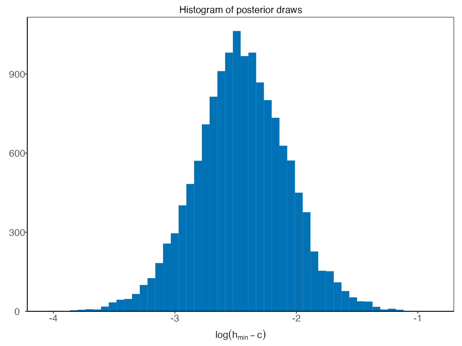
The bdrc package provides several tools to visualize the results from model objects which can give insight into the physical properties of the river at hand. For instance, the hyperparameter $c$ corresponds to the water elevation of zero discharge. To visualize the posterior of $c$ , we can write

> plot(gplm.fit, type = 'histogram', param = 'c')

Technically, instead of inferring $c$ directly, $h_{min}-c$ is inferred, where $h_{min}$ is the lowest water elevation value in the data. Since the parameter $h_{min}-c$ is strictly positive, a transformation $\zeta=log(h_{min}-c)$ is used for the Bayesian inference so that it has support on the real line. To plot the transformed posterior we write

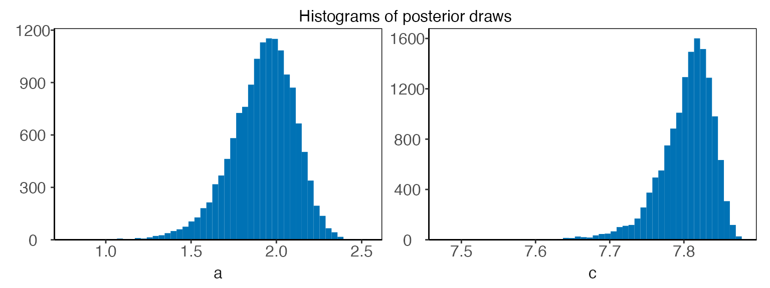
> plot(gplm.fit, type = 'histogram', param = 'c', transformed = TRUE)

The param argument can also be a vector containing multiple parameter names. For example, to visualize the posterior distributions of the parameters $a$ and $c$ , we can write

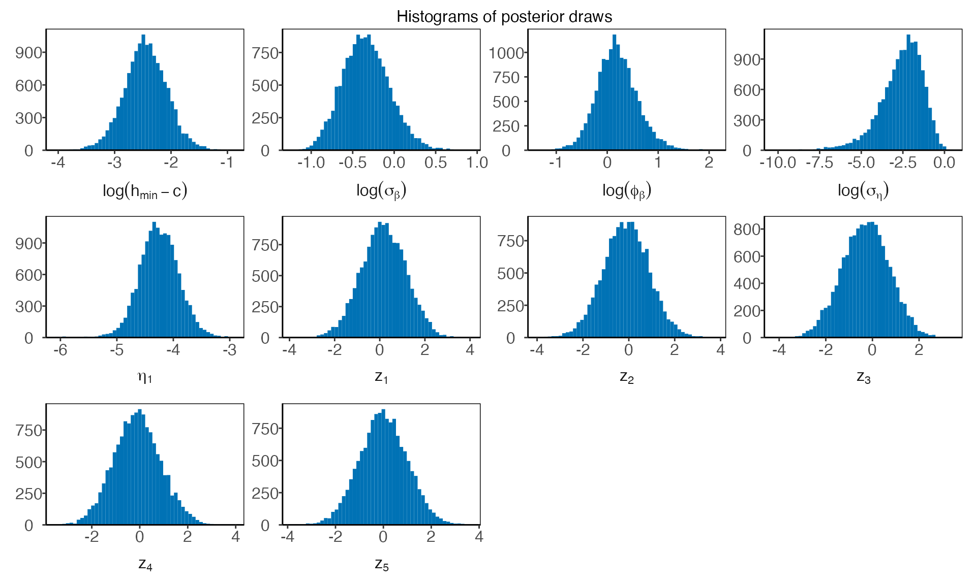
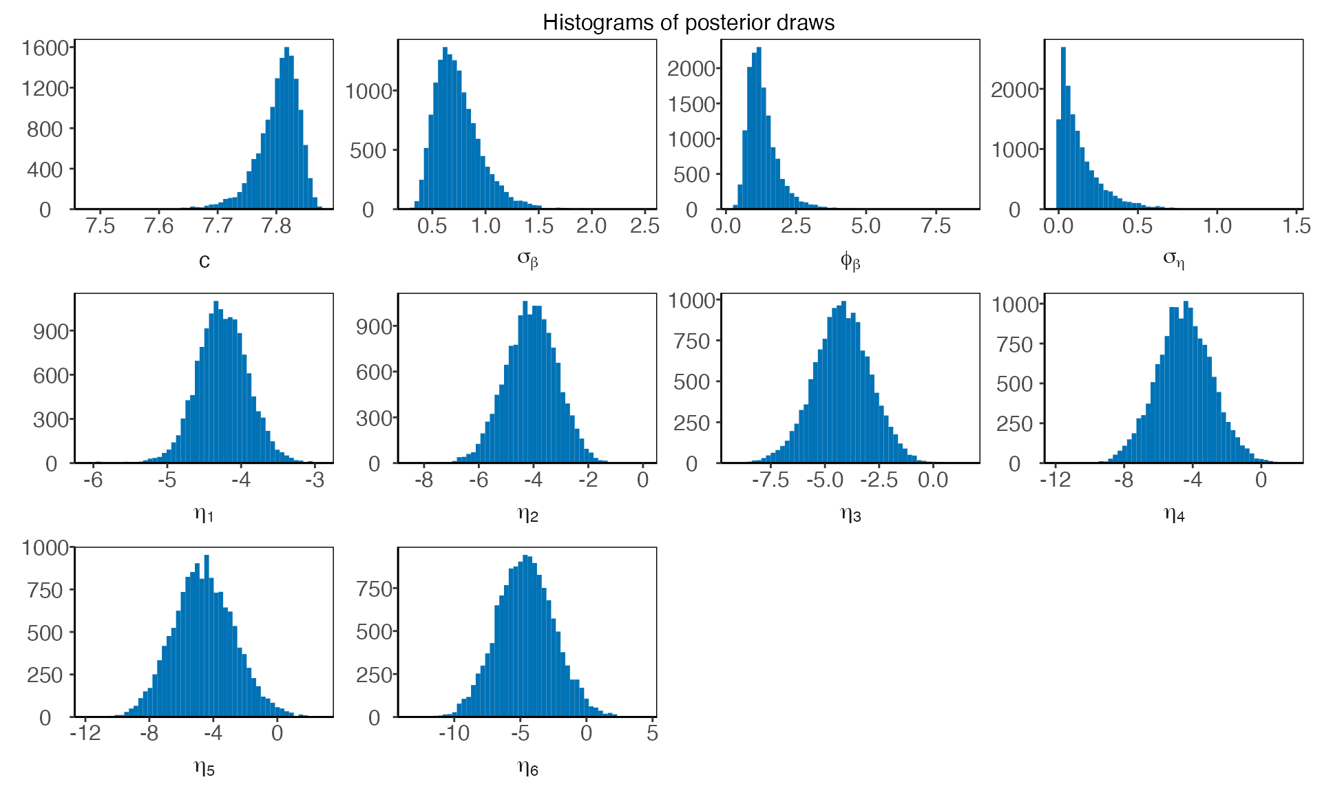
> plot(gplm.fit, type = 'histogram', param = c('a', 'c'))

There is a shorthand to visualize the hyperparameters all at once

> plot(gplm.fit, type = 'histogram', param = 'hyperparameters')

Similarly, writing "latent_parameters" plots the latent parameters in one plot. To plot the hyperparameters transformed on the same scale as in the Bayesian inference, we write

> plot(gplm.fit, type = 'histogram', param = 'hyperparameters', transformed = TRUE)

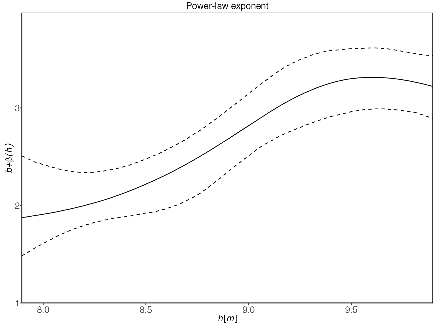
Finally, we can visualize the components of the model that are allowed (depending on the model) to vary with water elevation, that is, the power-law exponent, $f(h)$ , and the standard deviation of the error terms at the response level, $\sigma_{\varepsilon}(h)$ . Both gplm0 and gplm generalize the power-law exponent by modeling it as a sum of a constant term, $b$ , and Gaussian process, $\beta(h)$ , namely $f(h)=b+\beta(h)$ , where $\beta(h)$ is assumed to be twice differentiable with mean zero. On the other hand, plm and plm0 both model the power-law exponent as a constant by setting $\beta(h)=0$ , which gives $f(h)=b$ . We can plot the inferred power-law exponent with

> plot(gplm.fit, type = 'f')

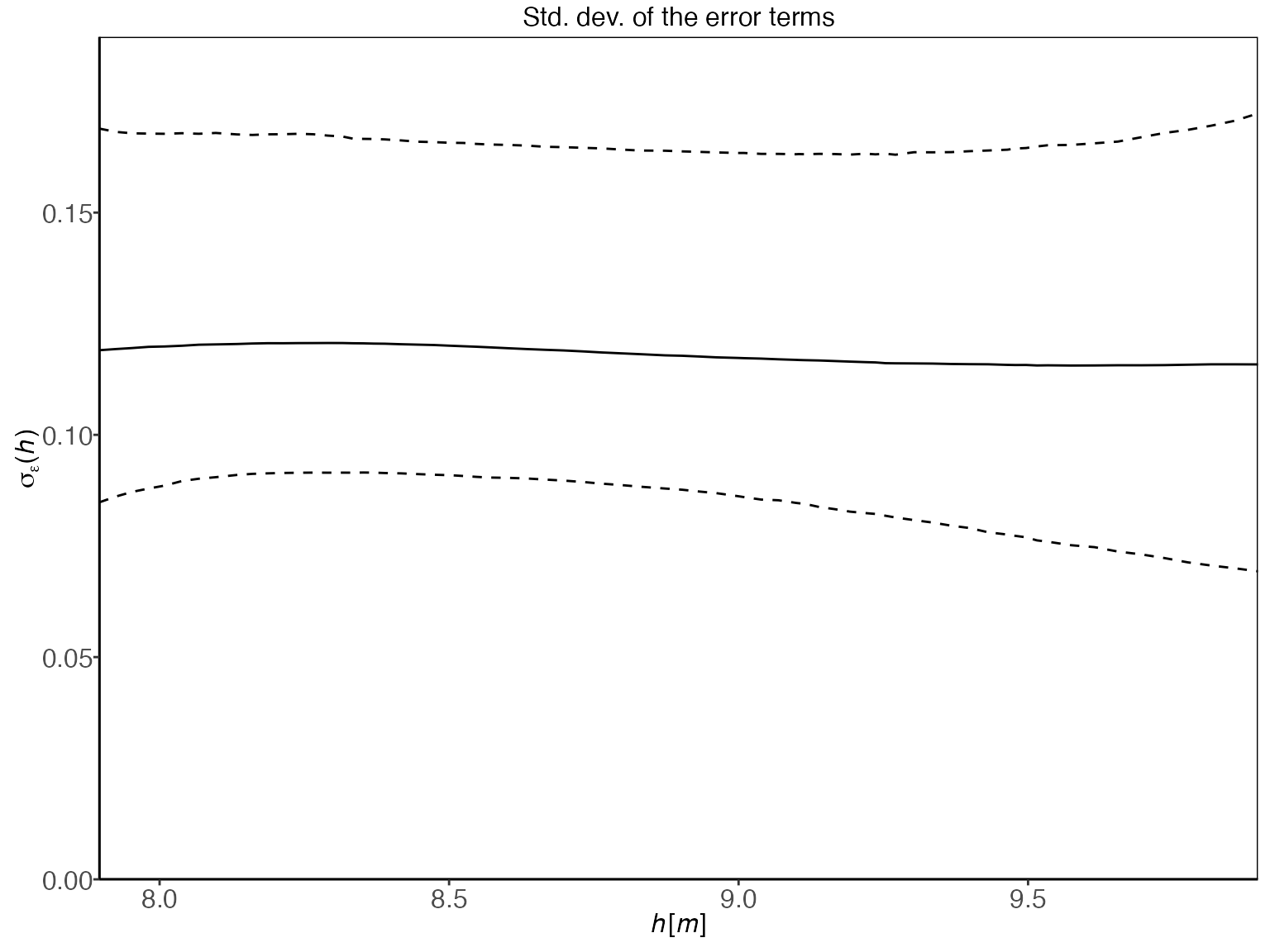
Both plm and gplm model the standard deviation of the error terms at the response level, $\sigma_{\varepsilon}(h)$ , as a function of water elevation, using B-splines basis functions, while plm0 and gplm0 model the standard deviation as a constant. We can plot the inferred standard deviation by writing

> plot(gplm.fit, type = 'sigma_eps')

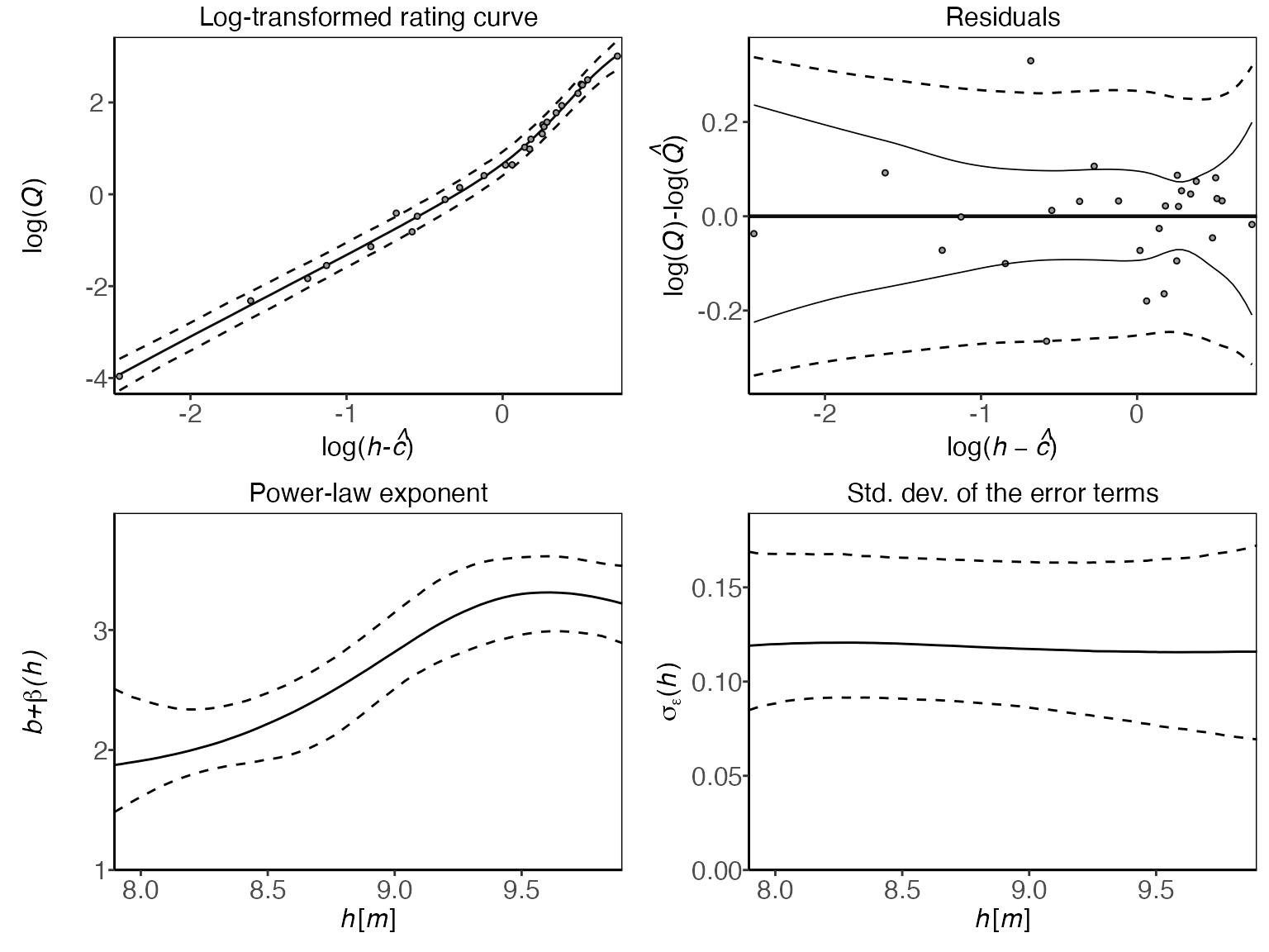
To get a visual summary of your model, the "panel" option in the plot type is useful:

> plot(gplm.fit, type = 'panel', transformed = TRUE)

Assessing model fit and convergence

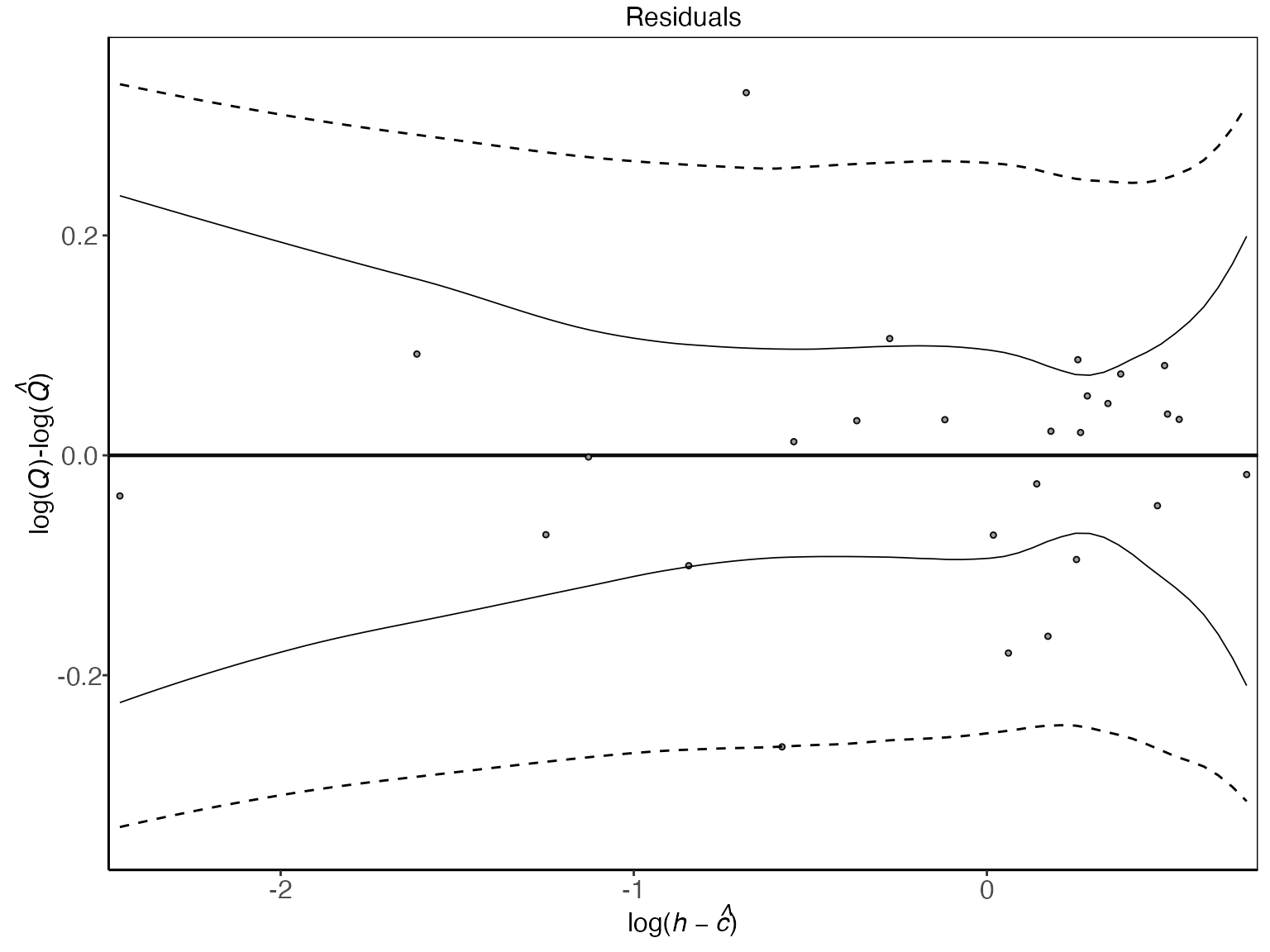
The package has several functions for convergence diagnostics of a bdrc model, most notably the residual plot, trace plots, autocorrelation plots, and Gelman-Rubin diagnostic plots. The log-residuals can be plotted with

> plot(gplm.fit, type = 'residuals')

The log-residuals are calculated by subtracting the posterior estimate (median) of the log-discharge, $log(\hat{Q})$ , from the observed log-discharge, $log(Q)$ . Additionally, the plot includes the 95% predictive intervals of $\log(Q)$ (- -) and 95% credible intervals for the expected value of $\log(Q)$ (—), the latter reflecting the rating curve uncertainty.

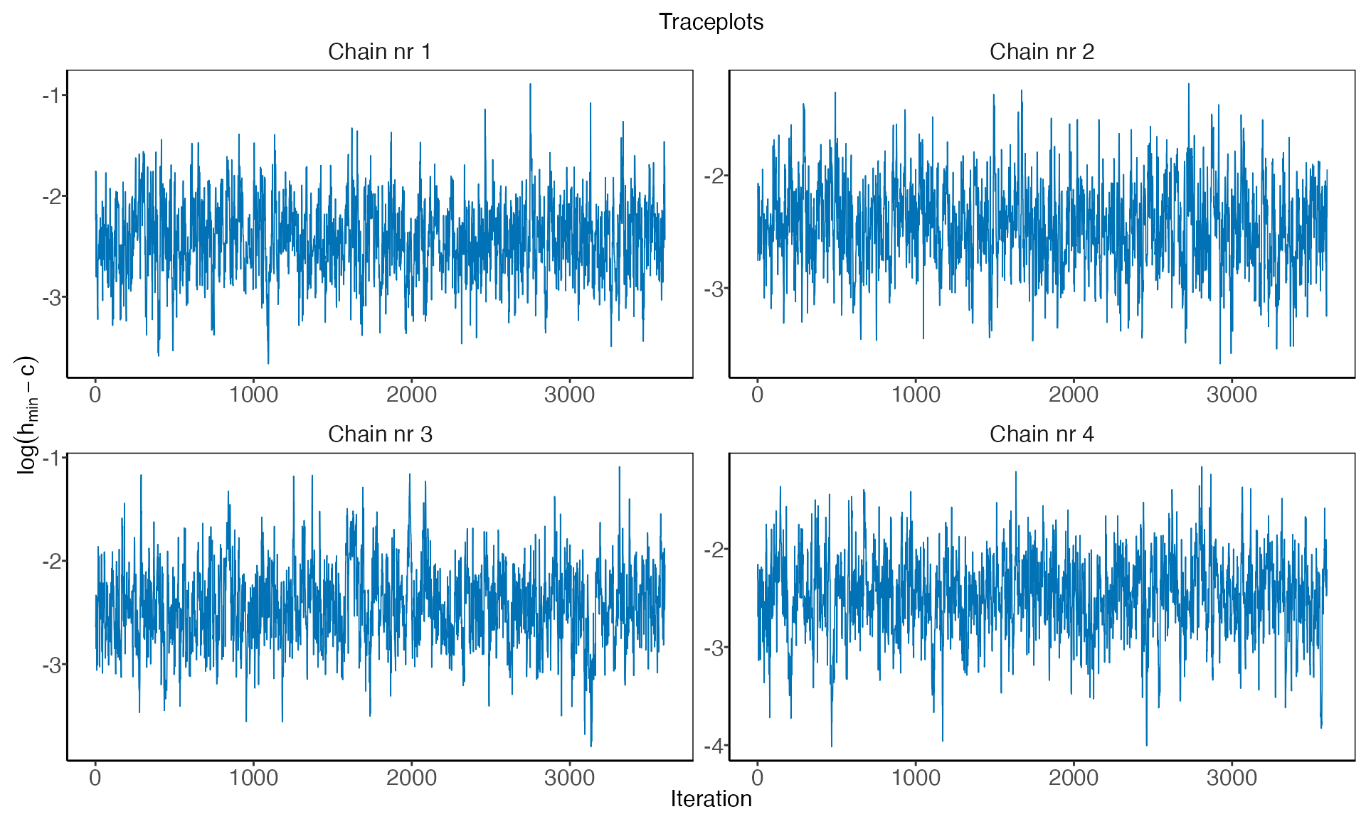
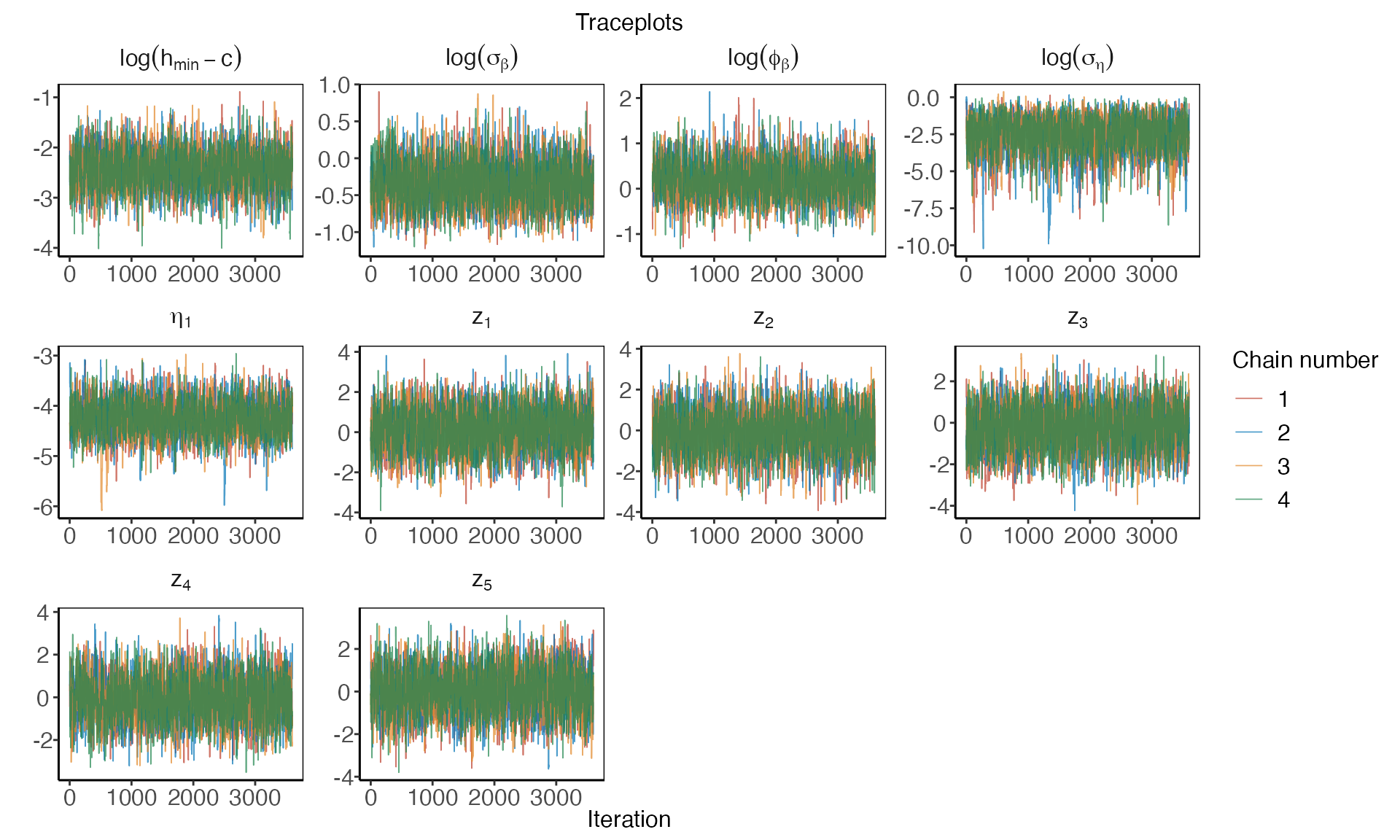
> plot(gplm.fit, type = 'trace', param = 'c', transformed = TRUE)

To plot a trace plot for all the transformed hyperparameters, we write

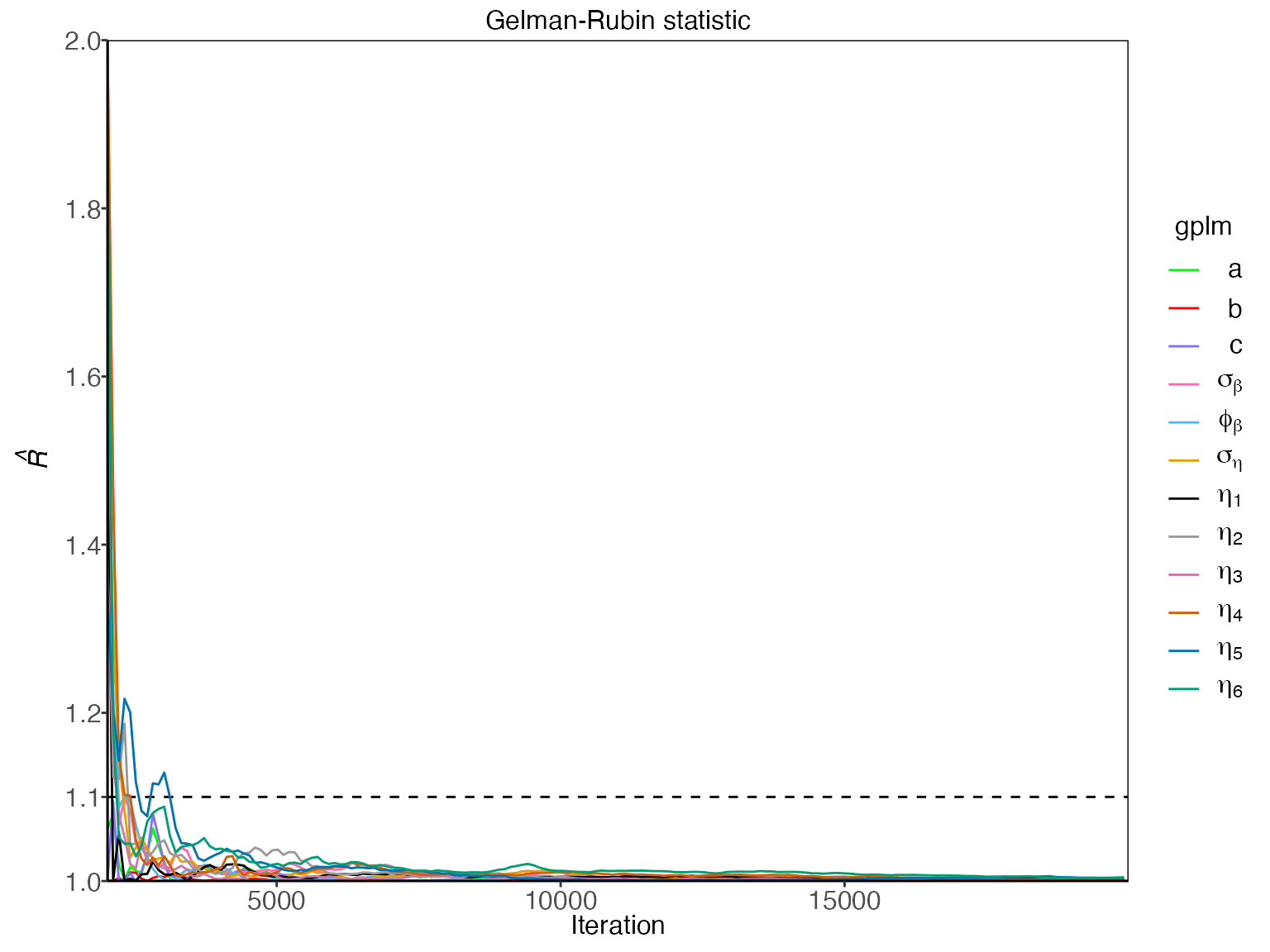
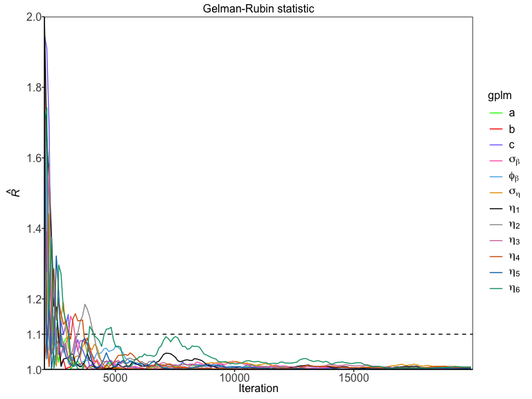
> plot(gplm.fit, type = 'trace', param = 'hyperparameters', transformed = TRUE)

To assess the mixing and convergence of the MCMC chains for each parameter, you can visualize the Gelman-Rubin statistic, $\hat{R}$ , as presented by Gelman and Rubin (1992) with:

> plot(gplm.fit, type = 'r_hat')

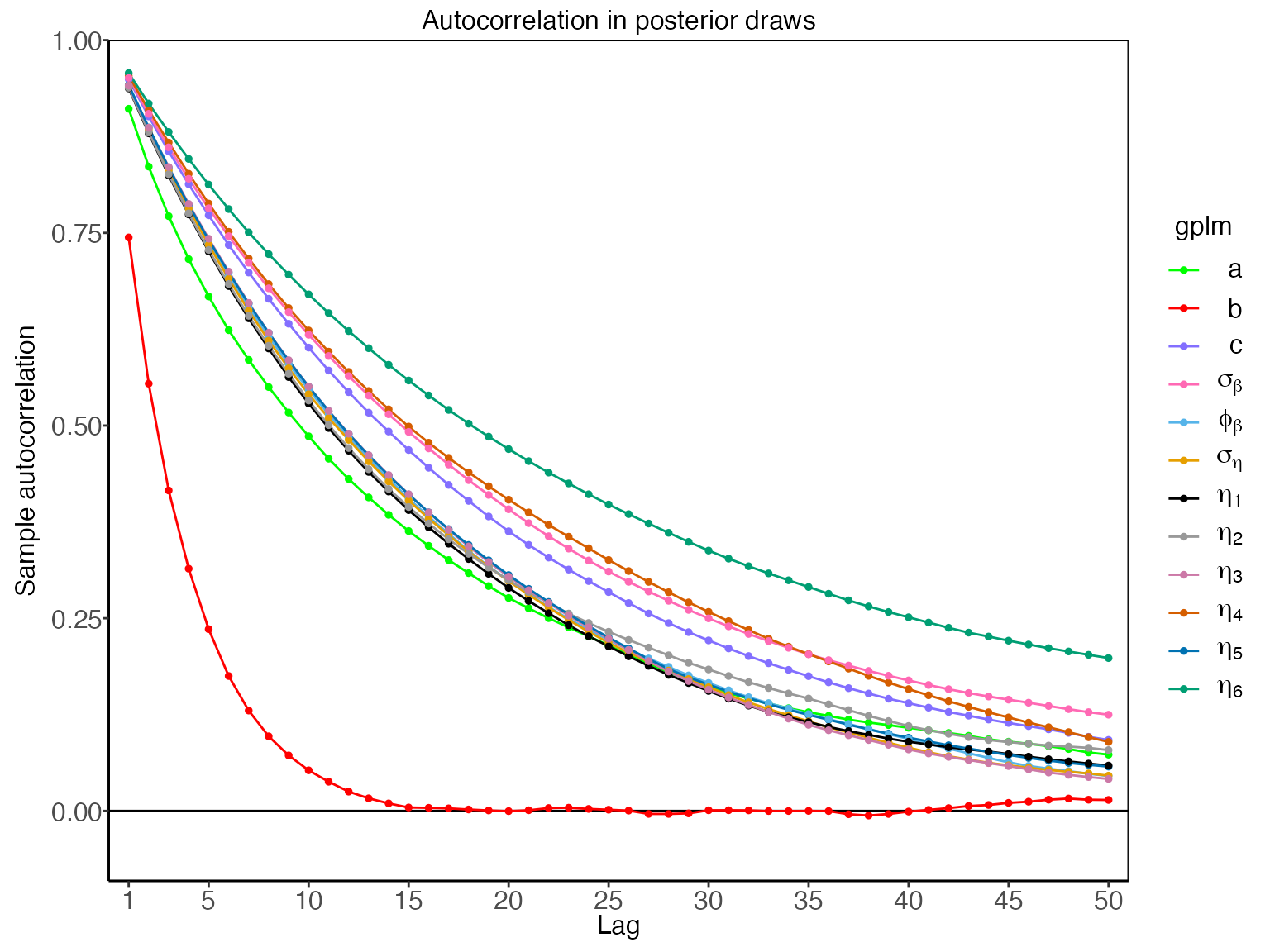
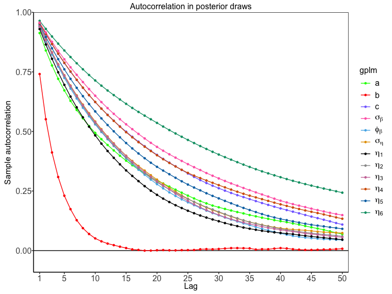
And finally, autocorrelation of parameters can be assessed with

> plot(gplm.fit, type = 'autocorrelation')

Customizing the models

There are ways to further customize the gplm function. In some instances, the parameter of zero discharge, $c$ , is known, and you might want to fix the model parameter to the known value. In addition, you might want to extrapolate the rating curve to higher water elevation values by adjusting the maximum water elevation. Assume 7.65 m is the known value of $c$ and you want to calculate the rating curve for water elevation values up to 10 m, then your function call would look like this

> gplm.fit.known_c <- gplm(Q ~ W, krokfors, c_param = 7.65, h_max = 10, parallel = FALSE)

Prediction for an equally spaced grid of water elevations

To get rating curve predictions for an equally spaced grid of water elevation values, you can use the predict function. Note that only values in the range from $c$ and h_max are accepted, as that is the range in which the Bayesian inference was performed

> h_grid <- seq(8, 8.2, by = 0.01)
> rating_curve_h_grid <- predict(gplm.fit, newdata = h_grid)
> print(rating_curve_h_grid)
#>       h      lower     median     upper
#> 1  8.00 0.06138853 0.08252241 0.1108601
#> 2  8.01 0.06708762 0.09009315 0.1207313
#> 3  8.02 0.07340524 0.09850833 0.1316830
#> 4  8.03 0.07972287 0.10692352 0.1426346
#> 5  8.04 0.08620981 0.11547827 0.1537808
#> 6  8.05 0.09363849 0.12480929 0.1660087
#> 7  8.06 0.10106716 0.13414031 0.1782366
#> 8  8.07 0.10861541 0.14364701 0.1906011
#> 9  8.08 0.11657272 0.15375469 0.2034327
#> 10 8.09 0.12453003 0.16386237 0.2162643
#> 11 8.10 0.13257127 0.17428375 0.2295414
#> 12 8.11 0.14080833 0.18543710 0.2438577
#> 13 8.12 0.14904540 0.19659045 0.2581741
#> 14 8.13 0.15728247 0.20774380 0.2724905
#> 15 8.14 0.16662200 0.21960922 0.2875367
#> 16 8.15 0.17662981 0.23190628 0.3030253
#> 17 8.16 0.18663761 0.24420333 0.3185138
#> 18 8.17 0.19681441 0.25692028 0.3351942
#> 19 8.18 0.20699699 0.26965158 0.3519154
#> 20 8.19 0.21718541 0.28270330 0.3691020
#> 21 8.20 0.22738677 0.29646391 0.3873183

References

Gelman, A., & Rubin, D. B. (1992). Inference from iterative simulation using multiple sequences, Statistical Science, 7(4), 457–472. doi: https://doi.org/10.1214/ss/1177011136