Visualize discharge rating curve model objects
Usage
# S3 method for class 'plm0'
autoplot(
  object,
  ...,
  type = "rating_curve",
  param = NULL,
  transformed = FALSE,
  title = NULL,
  xlim = NULL,
  ylim = NULL
)

# S3 method for class 'plm'
autoplot(
  object,
  type = "rating_curve",
  param = NULL,
  transformed = FALSE,
  title = NULL,
  xlim = NULL,
  ylim = NULL,
  ...
)

# S3 method for class 'gplm0'
autoplot(
  object,
  type = "rating_curve",
  param = NULL,
  transformed = FALSE,
  title = NULL,
  xlim = NULL,
  ylim = NULL,
  ...
)

# S3 method for class 'gplm'
autoplot(
  object,
  type = "rating_curve",
  param = NULL,
  transformed = FALSE,
  title = NULL,
  xlim = NULL,
  ylim = NULL,
  ...
)
Arguments
- object
An object of class "plm0", "plm", "gplm0" or "gplm".
- ...
Not used in this function
- type
A character denoting what type of plot should be drawn. Defaults to "rating_curve". Possible types are:
rating_curvePlots the rating curve.
rating_curve_meanPlots the posterior mean of the rating curve.
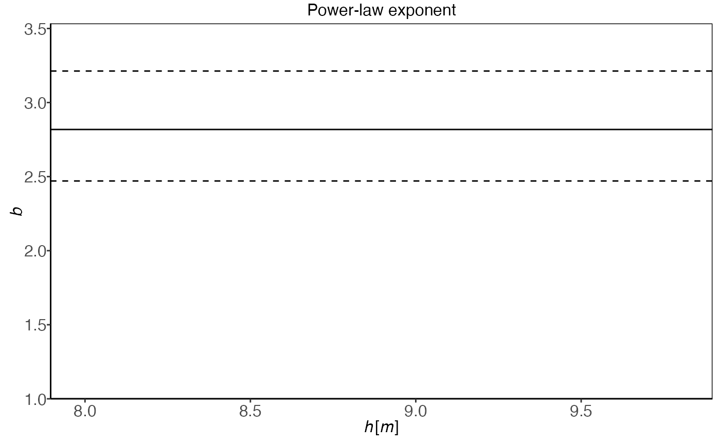
fPlots the power-law exponent.
betaPlots the random effect in the power-law exponent.
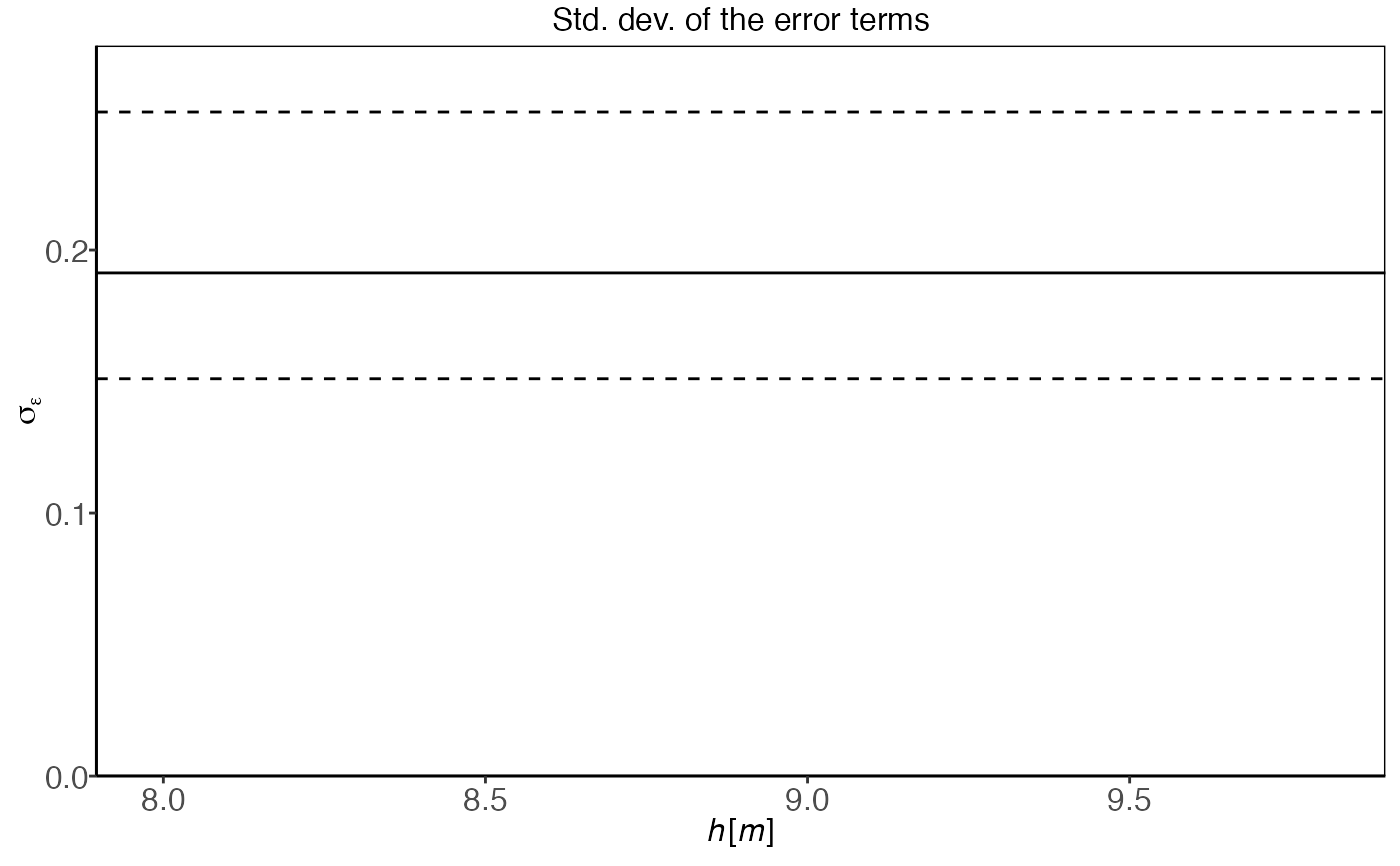
sigma_epsPlots the standard deviation on the data level.
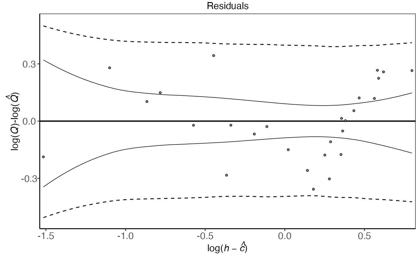
residualsPlots the log residuals.
tracePlots trace plots of parameters given in param.
histogramPlots histograms of parameters given in param.
- param
A character vector with the parameters to plot. Defaults to NULL and is only used if type is "trace" or "histogram". Allowed values are the parameters given in the model summary of x as well as "hyperparameters" or "latent_parameters" for specific groups of parameters.
- transformed
A logical value indicating whether the quantity should be plotted on a transformed scale used during the Bayesian inference. Defaults to FALSE.
- title
A character denoting the title of the plot.
- xlim
A numeric vector of length 2, denoting the limits on the x axis of the plot. Applicable for types "rating_curve", "rating_curve_mean", "f", "beta", "sigma_eps", "residuals".
- ylim
A numeric vector of length 2, denoting the limits on the y axis of the plot. Applicable for types "rating_curve", "rating_curve_mean", "f", "beta", "sigma_eps", "residuals".
Functions
autoplot(plm0): Autoplot method for plm0autoplot(plm): Autoplot method for plmautoplot(gplm0): Autoplot method for gplm0autoplot(gplm): Autoplot method for gplm
See also
plm0, plm, gplm0 and gplm for fitting a discharge rating curve and summary.plm0, summary.plm, summary.gplm0 and summary.gplm for summaries. It is also useful to look at spread_draws and gather_draws to work directly with the MCMC samples.
Examples
# \donttest{
library(ggplot2)
data(krokfors)
set.seed(1)
plm0.fit <- plm0(Q~W,krokfors,num_cores=2)
#> Progress:
#> Initializing Metropolis MCMC algorithm...
#> Multiprocess sampling (4 chains in 2 jobs) ...
#>
#> MCMC sampling completed!
#>
#> Diagnostics:
#> Acceptance rate: 36.09%.
#> ✔ All chains have mixed well (Rhat < 1.1).
#> ✔ Effective sample sizes sufficient (eff_n_samples > 400).
autoplot(plm0.fit)
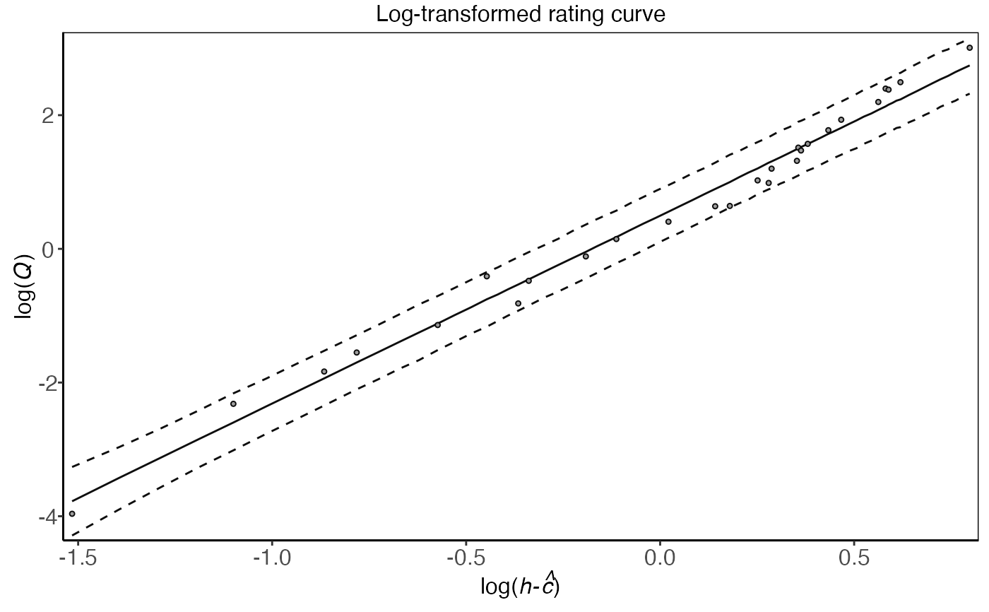
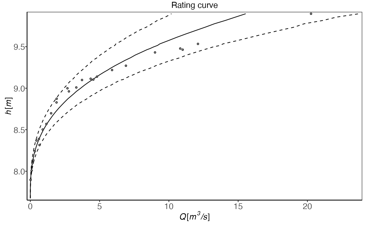 autoplot(plm0.fit,transformed=TRUE)
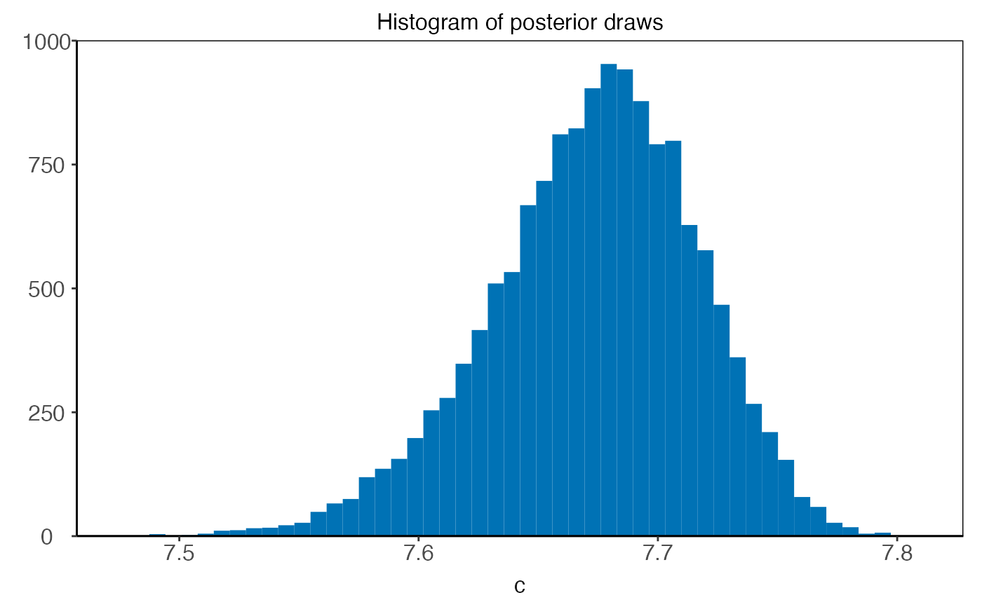
 autoplot(plm0.fit,type='histogram',param='c')
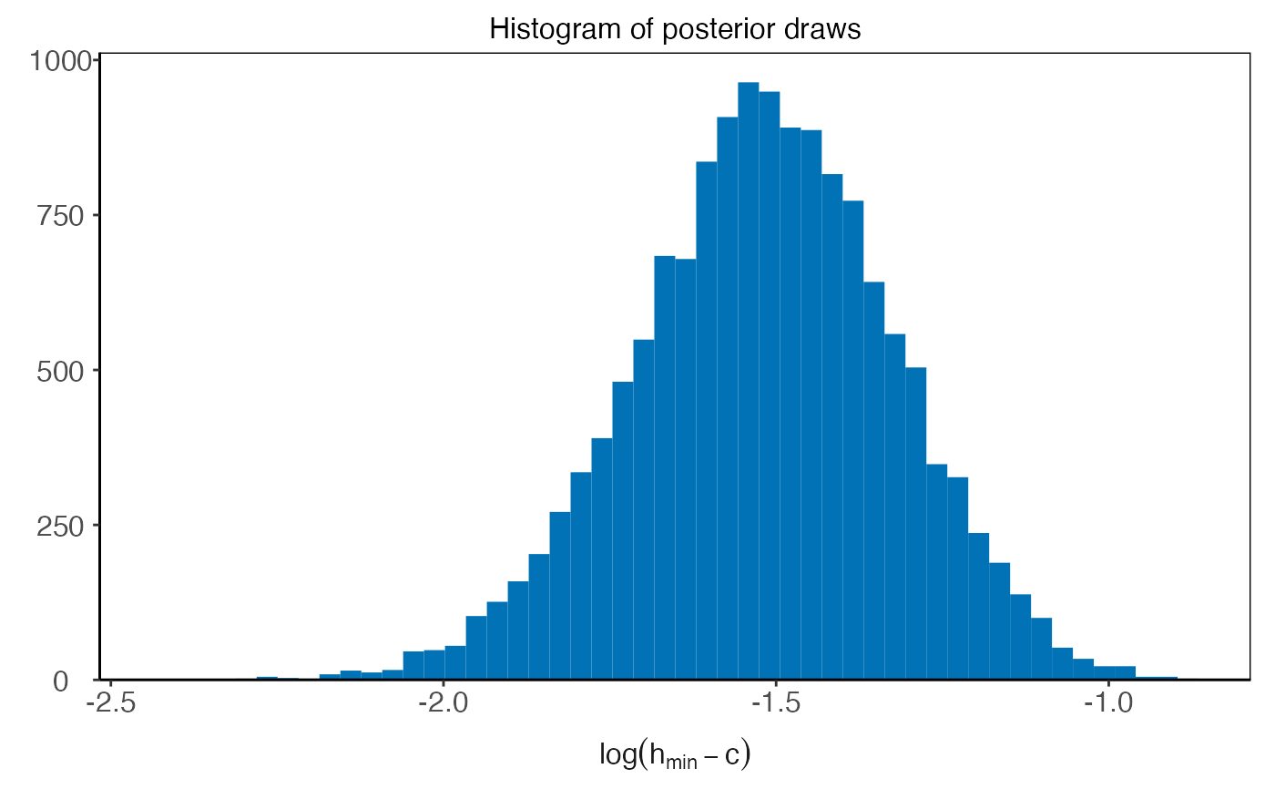
 autoplot(plm0.fit,type='histogram',param='c',transformed=TRUE)
 autoplot(plm0.fit,type='histogram',param='hyperparameters')
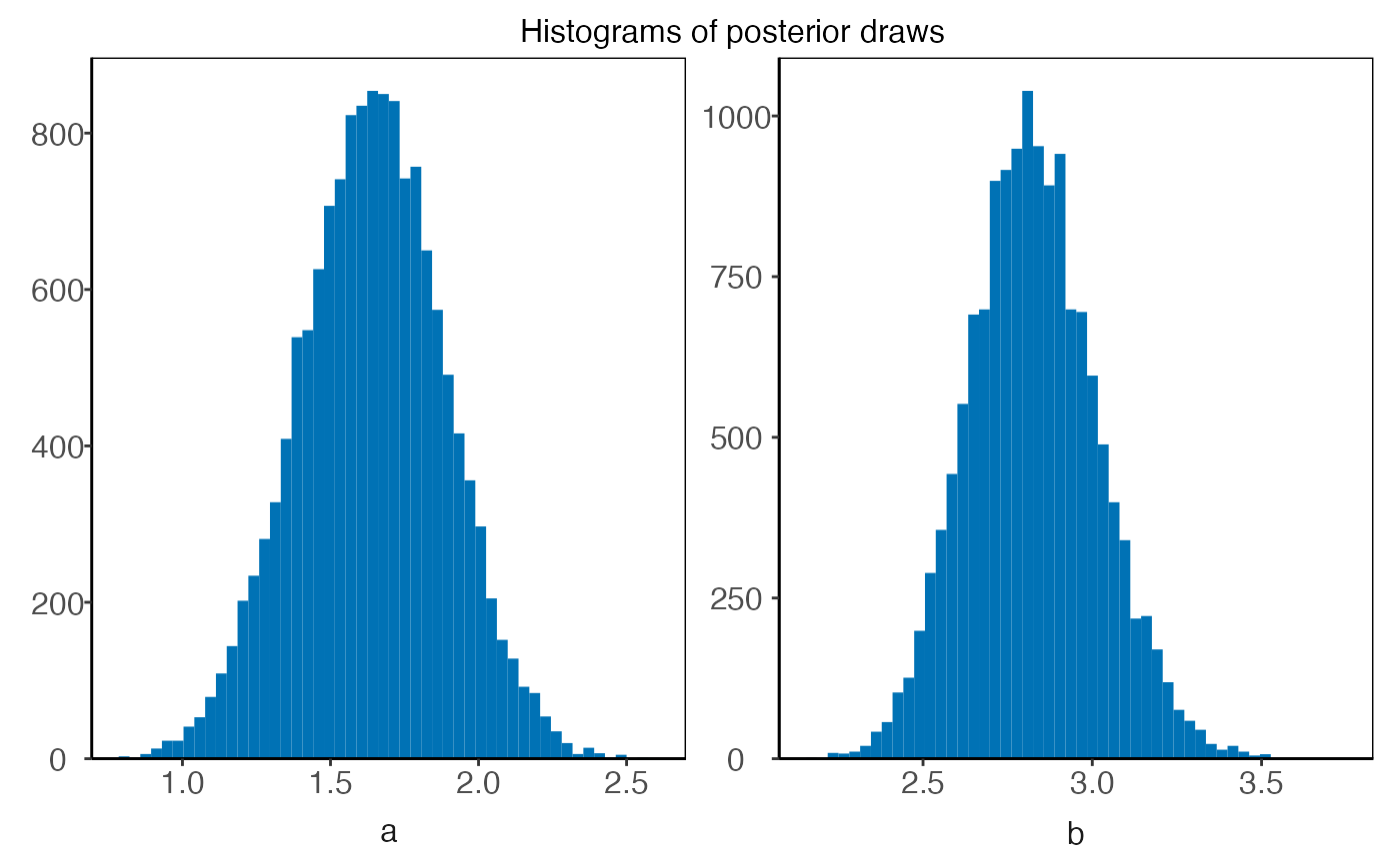
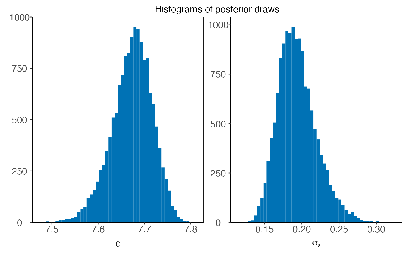 autoplot(plm0.fit,type='histogram',param='latent_parameters')
 autoplot(plm0.fit,type='residuals')
 autoplot(plm0.fit,type='f')
 autoplot(plm0.fit,type='sigma_eps')
 # }
# }